library(werptoolkitr)
library(dplyr)
library(ggplot2)
library(patchwork)Spatial aggregation
Overview
We will often have spatial data that we want to aggregate into larger scales. We therefore want a set of functions that allow us to read in data, specify the larger units into which it gets aggregated and the functions to use to do that aggregation. Further, there is clear need to handle grouping, most obviously for scenarios, but we also need to keep theme groupings separated during spatial aggregation steps.
There is a standalone spatial aggregator spatial_aggregate, which I demonstrate here, along with multi_aggregate, which wraps both spatial_aggregate and theme_aggregate to allow interleaved aggregaton steps in a standardised format. This document focuses on spatial aggregation, while theme aggregation and interleaved spatial and theme aggregation are demonstrated in separate notebooks, allowing us to dig a little deeper into how each component works.
We often will want to only perform a single spatial aggregation (e.g. from gauges to sdl units), but there are instances where that isn’t true- perhaps we want to aggregate from sdl units to states or the basin. Thus, I demonstrate multi-step spatial aggregation, including the situation where aggregation units (polygons) are not nested, as would be the case for sdl units and states, for example. Even if some of the steps in this demonstration aren’t particularly interesting now, they allow us to develop the general process that can accept any set of polygons we want to aggregate into from any other spatial data.
This document delves fairly in-depth into capabilities, including things like argument types and how they relate to other functions and permit certain tricks. Not all of these will be used or needed to understand by most users- typically there will be a set of aggregation steps fed to multi_aggregate and that will be that. This sort of simpler setup is shown in the combined aggregation notebook and the full-toolkit runs. But it is helpful to document them for when they are needed. See the syntax notebook for a detailed look at argument construction for various purposes. Here, we use that syntax to demonstrate how the spatial aggregation works and the different ways it can be done.
Inputs
We will need to be able to accept inputs at arbitrary aggregation levels (theme, spatial, or temporal). In other words, the spatial aggregation should aggregate any input spatial data into any set of spatial units, whatever that input data represents. The multi_aggregate function runs without spatial info until it reaches a step calling for spatial aggregation, at which point that data must be spatial. Beyond this requirement, multi_aggregate doesn’t care what theme or spatial scale that input data is- e.g. we could give it Objectives already at the Catchment scale, and then use it to move up.
Note: in some cases, the definitions for outcomes along the ‘Objective’ axis are defined spatially; for example, the definition of Specific_objectives might vary between planning units. However, these are the scale at which definitions of outcomes change, not the scale at which those outcomes must be assessed. For example, just because Specific_objectives are differently defined between planning units, we can still scale them up in space from gauge to basin, with no reference to planning unit.
For this demonstration, we start with gauge-referenced data at the env_obj theme scale.
Demonstration setup
First, we need to provide a set of paths to point to the input data, in this case the outputs from the EWR tool for the small demonstration, created by a controller notebook. Spatial units could be any arbitrary polygons, but we use those provided by {werptoolkitr} for consistency, which also provides the spatial locations of the gauges in bom_basin_gauges.
project_dir <- file.path('more_scenarios')
ewr_results <- file.path(project_dir, 'module_output', 'EWR')
Theme aggregated inputs
The multi_aggregate function can combine theme and spatial aggregation, but because I want this document to demonstrate spatial aggregation, I have split up the process to be clear what is happening. First, we do a theme aggregation to get to the desired Theme level to feed to spatial.
Before any aggregation, we need to read the data in and make it spatial (gauge2geo pairs gauge numbers with locations provided in the geopath argument inside prep_ewr_agg. Note that this prep step is wrapped in read_and_agg, reducing user input. I show it here so we can more clearly see what is happening.
sumdat <- prep_ewr_agg(ewr_results, type = 'summary', geopath = bom_basin_gauges)Define simple theme aggregation lists to get to env_obj level, assuming that any pass on ewr_code_timing yields a pass for ewr_code and ewr_codes are averaged into env_obj. More complexity for the theme aggregations are shown in the theme notebook.
themeseq <- list(c('ewr_code_timing', 'ewr_code'),
               c('ewr_code', "env_obj"))

funseq <- list(c('CompensatingFactor'),
               c('ArithmeticMean'))
Perform that simple theme aggregation so we have some test data. Since edges are only relevant for theme aggregation, make them in the call. This and everything that follows could be done with interleaved theme and spatial sequences starting with themeseq and funseq fed to multi_aggregate, but here I split them apart to better accentuate the spatial aggregation.
simpleThemeAgg <- multi_aggregate(dat = sumdat,
                         causal_edges = make_edges(causal_ewr, themeseq),
                         groupers = c('scenario', 'gauge'),
                         aggCols = 'ewr_achieved',
                         aggsequence = themeseq,
                         funsequence = funseq)
simpleThemeAgg
This provides a spatially-referenced (to gauge) theme-aggregated tibble to use to demonstrate spatial aggregation. Note that this has the gauge (spatial unit), but also two groupings that we want to preserve when we spatially aggregate- scenario and the current level of theme grouping, env_obj.
Spatial inputs (polygons)
Spatial aggregation requires polygons to aggregate into, and we want the capability to do that several times. The user can read in any desired polygons with sf::read_sf(path/to/polygon.shp), but here we use those provided in the standard set with {werptoolkitr}. We’ll use SDL units, catchments (from cewo), and the basin to show how the aggregation can have multiple steps with polygons that may not be nested (though care should be taken when that is the case).
Demonstrations
We’ll now use that input data to demonstrate how to do the spatial aggregation, demonstrate capabilities and options provided by the function, and provide additional information useful to the user.
Single aggregation
We might just want to aggregate spatially once. We can do this simply by passing the input data (anything spatial, in this case simpleThemeAgg), a set of polygons, and providing a length-one funlist. In this simple case, we just use a bare function name, here the custom ArithmeticMean which is just a simple wrapper of mean with na.rm = TRUE. Any function can be passed this way, custom or in-built, provided it has a single argument. More complex situations are given below.
Note that the aggCols argument is ends_with(original_name) to reference the original name of the column of values- it may have a long name tracking its aggregation history, so we give it the tidyselect ends_with to find the column. More generally, both aggCols and groupers can take any tidyselect syntax or bare names or characters.
obj2poly <- spatial_aggregate(dat = simpleThemeAgg,
                             to_geo = sdl_units,
                             groupers = 'scenario',
                             aggCols = ends_with('ewr_achieved'),
                             funlist = ArithmeticMean,
                             keepAllPolys = TRUE)
obj2poly
Note that that has a horribly long name tracking the aggregation history, and has lost the theme levels- e.g. the different env_objs are no longer there and were all averaged together. The multi_aggregate function automatically handles this preservation, but spatial_aggregate is more general, and does not make any assumptions about the grouping structure of the data. Thus, to keep the env_obj groupings (as we should, otherwise we’re inadvertently theme-aggregating over all of them), we need to add env_obj to the groupers argument.
obj2poly <- spatial_aggregate(dat = simpleThemeAgg,
                             to_geo = sdl_units,
                             groupers = c('scenario', 'env_obj'),
                             aggCols = ends_with('ewr_achieved'),
                             funlist = ArithmeticMean,
                             keepAllPolys = TRUE)
obj2poly
A quick plot shows what we’re dealing with. We’ll simplify the names and choose a subset of the environmental objectives.
There are many built-in plotting options in the toolkit, which we will use shortly. First, though a quick ggplot to see what those standardised plot functions start with.
# The name is horrible, so change it.
obj2poly %>%
  rename(ewr_achieved = spatial_ArithmeticMean_env_obj_ArithmeticMean_ewr_code_CompensatingFactor_ewr_achieved) %>%
  filter(grepl('^EF', env_obj)) %>%
ggplot(aes(fill = ewr_achieved)) +
  geom_sf() +
  facet_grid(scenario~env_obj) +
  theme(legend.position = 'bottom')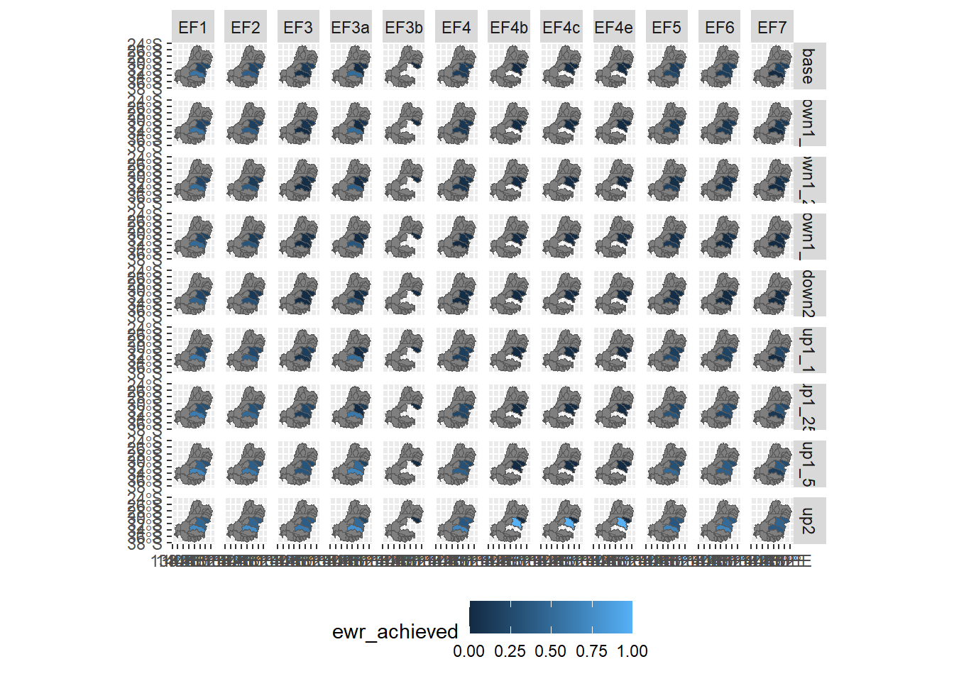
Moving forward, we’ll use the built-in plotting functions to keep consistent with the rest of the project.
scene_pal <- make_pal(unique(simpleThemeAgg$scenario), palette = 'ggsci::nrc_npg', refvals = 'base', refcols = 'black')obj2poly %>%
rename(ewr_achieved = spatial_ArithmeticMean_env_obj_ArithmeticMean_ewr_code_CompensatingFactor_ewr_achieved) %>%
filter(grepl('^EF[1-3]', env_obj)) %>%
plot_outcomes(y_col = 'ewr_achieved',
y_lab = 'Arithmetic Mean',
x_col = 'map',
colorgroups = NULL,
colorset = 'ewr_achieved',
pal_list = list('scico::berlin'),
facet_col = 'env_obj',
facet_row = 'scenario',
scene_pal = scene_pal,
sceneorder = c('down2', 'base', 'up2'))
Multiple spatial levels
There are a number of polygon layers we might want to aggregated into in addition to SDL units, e.g. resource plan areas, hydrological catchments, or the whole basin. We can aggregate directly into them just as we have here for SDL units. However, we might also want to have several levels of spatial aggregation, which may be nested or nearly so, e.g. from SDL units to the basin, or may be nonnested, e.g. from SDL units to catchments. Typically, this would happen with intervening theme aggregations, as in the interleaved example. The aggregation process for multiple spatial levels is similar whether or not the smaller levels nest into the larger, but more care should be taken (and more explanation is needed) in the nonnested case.
Note that there is an exception to the ‘vector arguments must be attached to the data’ rule, in that an area column is always created, making it available for things like area-weighted means.
Aggregating from SDL units to cewo valleys requires addressing issues of overlaps among the various polygons. As such, it makes a good test case that catches issues with the intersection of polygons that might not happen with a simpler set of polygons Figure 1 .
overlay_cewo_sdl <- ggplot() +
  geom_sf(data = sdl_units, aes(fill = SWSDLName), color = NA, alpha = 0.5) +
  geom_sf(data = cewo_valleys, aes(color = ValleyName), fill = NA) +
  theme(legend.position = 'none')

valleys <- ggplot() +
  geom_sf(data = cewo_valleys, aes(color = ValleyName), fill = 'white') +
  theme(legend.position = 'none')

sdls <- ggplot() +
  geom_sf(data = sdl_units, aes(fill = SWSDLName), alpha = 0.5) +
  theme(legend.position = 'none')

valleys + sdls + overlay_cewo_sdl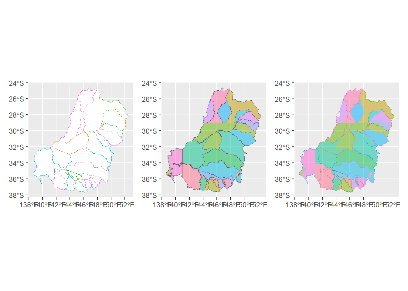
To aggregate from one set of polygons into the other, we need to split them up and aggregate in a way that respects area and borders. In other words, if we have a polygon that lays across two of the next level up, we want to only include the bits that overlap into that next level up. Under the hood, we use sf::st_intersection, which splits the polygons to make a new set of nonoverlapping polygons. Then we can use these pieces to aggregate into the higher level. This aggregation should carefully consider area- things like means should be area-weighted, and things like sums, minima, and maxima should be thought about carefully- if the lower ‘from’ data are already sums, for example, an area weighting might make sense to get a proportion of the sum, but this is highly dependent on the particular sequence of aggregation. For other functions like minima and maxima, area-weighting may or may not be appropriate, and so careful attention should be paid to constructing the aggregation sequence and custom functions may be involved.
The intersection of sdl_units and cewo_valleys chops up sdl_units so there are unique polygons for each sdl unit - valley combination.
joinpolys <- st_intersection(sdl_units, cewo_valleys)
joinpolys
To better see the many-to-many chopping we get with this particular pair of intersecting shapefiles, we can isolate an SDL unit (Victorian Murray) and see that it contains bits of 8 catchments. Likewise, the Loddon catchment contains bits of 4 SDL units Figure 2 .
nvorig <- ggplot() +
  geom_sf(data = dplyr::filter(sdl_units, SWSDLName == "Victorian Murray"))

nvpostjoin <- ggplot() +
  geom_sf(data = dplyr::filter(joinpolys,
                        SWSDLName == "Victorian Murray"),
          aes(fill = ValleyName))

avorig <- ggplot() +
  geom_sf(data = dplyr::filter(cewo_valleys, ValleyName == 'Loddon'))

avpostjoin <- ggplot() +
  geom_sf(data = dplyr::filter(joinpolys,
                        ValleyName == 'Loddon'),
          aes(fill = SWSDLName))

(nvorig + nvpostjoin)/(avorig + avpostjoin)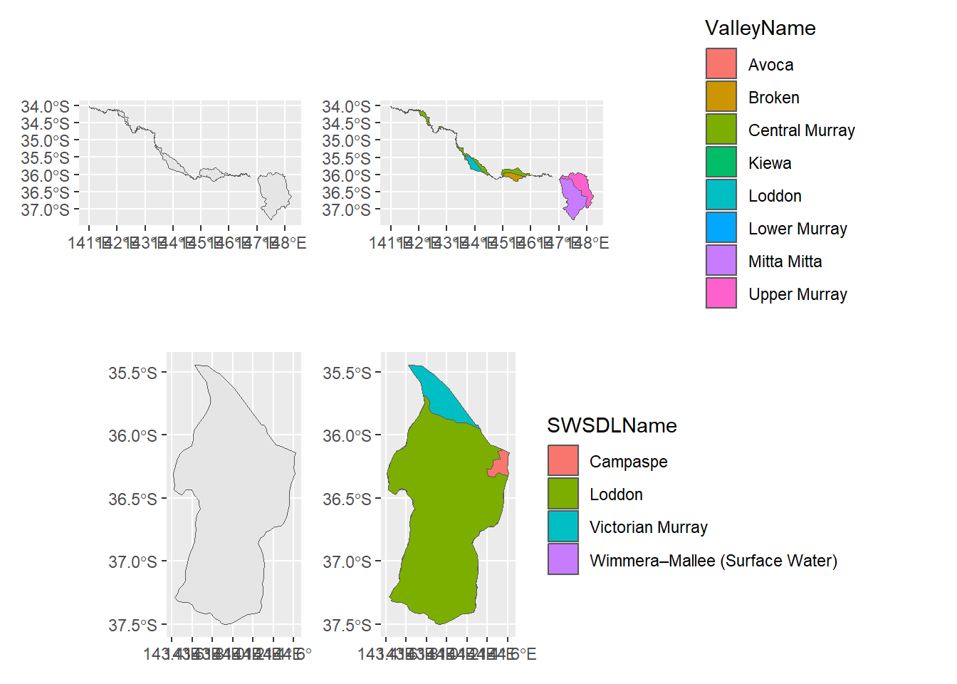
As a simple example, we could again do a one-off aggregation from a polygon to another polygon using spatial_aggregate. Here, we could use the obj2poly aggregation into SDL units created above as the starting point.
simplepolypoly <- spatial_aggregate(dat = obj2poly,
                 to_geo = cewo_valleys,
                 groupers = c('scenario', 'env_obj'),
                 aggCols = 'ewr_achieved',
                 funlist = mean,
                 na.rm = TRUE,
                 keepAllPolys = TRUE,
                 failmissing = FALSE)
simplepolypoly
As with all sequential aggregations, this approach works but can be very ad-hoc and easy to forget theme-axis grouping. Instead, just like with interleaved theme and space, we can pass a list giving the aggregation sequence to multi_aggregate.
Passing a list
We can use multi_aggregate to aggregate through a list of polygon sets, here sdl units to cewo valleys to the basin.
First, set up a list of the spatial aggregation steps, defined by the polygon sets and aggregation functions. As usual, multiple aggregation functions can happen at each stage, and they can be characters or named lists with arguments (the weighted mean needs to be a default). Now, we’re taking advantage of the auto-calculated area of each polygon chunk for the weighted mean.
note the rlang::quo to make this work with dplyr 1.1 and above as in syntax.
glist <- list(sdl_units = sdl_units, catchment = cewo_valleys, mdb = basin)

funlist <- list(c('ArithmeticMean', 'LimitingFactor'),
                rlang::quo(list(wm = ~weighted.mean(., area, na.rm = TRUE))),
                rlang::quo(list(wm = ~weighted.mean(., area, na.rm = TRUE))))
multispat <- multi_aggregate(dat = simpleThemeAgg,
causal_edges = themeedges,
groupers = c('scenario', 'env_obj'),
aggCols = 'ewr_achieved',
aggsequence = glist,
funsequence = funlist)By default, that returns only the final outcome, here the basin scale and with the aggregation history in column names so we are sure of what the values represent Figure 3 . That does not make a very readable legend, but we can rename it manually and tracking the meaning is very important.
multispat %>%
  filter(grepl('^NF[1-3]', env_obj)) %>%
ggplot() +
  geom_sf(aes(fill = mdb_wm_catchment_wm_sdl_units_ArithmeticMean_env_obj_ArithmeticMean_ewr_code_CompensatingFactor_ewr_achieved)) +
  facet_grid(env_obj~scenario) + theme(legend.position = 'bottom')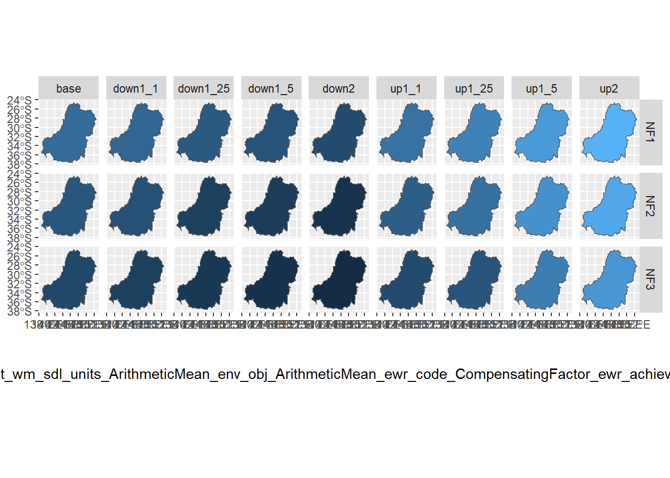
Saveintermediate and namehistory
We might only want the final outcome as above, but we also might want all the steps (just as we did for the theme. Making the history in columns keeps the names easier to use, though it uses more memory. I am going to do something I shouldn’t here, and change the column ‘env_obj_ArithmeticMean_ewr_code_CompensatingFactor_ewr_achieved’ to ‘ewr_achieved’. That’s for readability and because here we’re using namehistory = FALSE to track the history in columns. If we were truly doing this analysis, the theme-axis aggregations in simpleThemeAgg would be included in the aggsequence, and so those steps would also be handled with aggsequence columns.
simpleclean <- simpleThemeAgg %>%
  rename(ewr_achieved = env_obj_ArithmeticMean_ewr_code_CompensatingFactor_ewr_achieved)

multispatb <- multi_aggregate(dat = simpleclean,
                              causal_edges = themeedges,
                              groupers = c('scenario', 'env_obj'),
                              aggCols = 'ewr_achieved',
                              aggsequence = glist,
                              funsequence = funlist,
                              saveintermediate = TRUE,
                              namehistory = FALSE)
That final list item is scenario * aggfun1*aggfun2*aggfun3*env_obj long, e.g. it has a row for each scenario and env_obj by aggregation function, and the aggregation functions are factorial- both the aggregations at step 1 are subsequently aggregated at each of the following steps.
length(unique(multispatb$mdb$scenario)) *
length(unique(multispatb$mdb$aggfun_1)) *
length(unique(multispatb$mdb$aggfun_2)) *
length(unique(multispatb$mdb$aggfun_3)) *
  length(unique(multispatb$mdb$env_obj))
[1] 828nrow(multispatb$mdb)[1] 828Now we can more easily analyse the output, but it’s bigger. The three spatial levels plus the input can all be mapped. We’ll cut it down to a single env_obj for clarity and use the comparer standard plots, with a common set of limits. We have to choose one of the aggfun_1 values.
l1 <- multispatb$simpleclean %>%
  filter(grepl('^NF1', env_obj)) %>%
  plot_outcomes(y_col = 'ewr_achieved',
                x_col = 'map',
                colorgroups = NULL,
                colorset = 'ewr_achieved',
                pal_list = list('scico::berlin'),
                facet_col = 'scenario',
                facet_row = 'env_obj',
                scene_pal = scene_pal,
                sceneorder = c('down2', 'base', 'up2'),
                underlay_list = 'basin',
                setLimits = c(0,1))

l2 <- multispatb$sdl_units %>%
  filter(grepl('^NF1', env_obj) &
           aggfun_1 == 'ArithmeticMean') %>%
  plot_outcomes(y_col = 'ewr_achieved',
                x_col = 'map',
                colorgroups = NULL,
                colorset = 'ewr_achieved',
                pal_list = list('scico::berlin'),
                facet_col = 'scenario',
                facet_row = 'env_obj',
                scene_pal = scene_pal,
                sceneorder = c('down2', 'base', 'up2'),
                underlay_list = 'basin',
                setLimits = c(0,1))

l3 <- multispatb$catchment %>%
  filter(grepl('^NF1', env_obj) &
           aggfun_1 == 'ArithmeticMean') %>%
  plot_outcomes(y_col = 'ewr_achieved',
                x_col = 'map',
                colorgroups = NULL,
                colorset = 'ewr_achieved',
                pal_list = list('scico::berlin'),
                facet_col = 'scenario',
                facet_row = 'env_obj',
                scene_pal = scene_pal,
                sceneorder = c('down2', 'base', 'up2'),
                underlay_list = 'basin',
                setLimits = c(0,1))

l4 <- multispatb$mdb %>%
  filter(grepl('^NF1', env_obj) &
           aggfun_1 == 'ArithmeticMean') %>%
  plot_outcomes(y_col = 'ewr_achieved',
                x_col = 'map',
                colorgroups = NULL,
                colorset = 'ewr_achieved',
                pal_list = list('scico::berlin'),
                facet_col = 'scenario',
                facet_row = 'env_obj',
                scene_pal = scene_pal,
                sceneorder = c('down2', 'base', 'up2'),
                underlay_list = 'basin',
                setLimits = c(0,1))
l1 / l2 / l3 / l4 + plot_layout(guides = 'collect')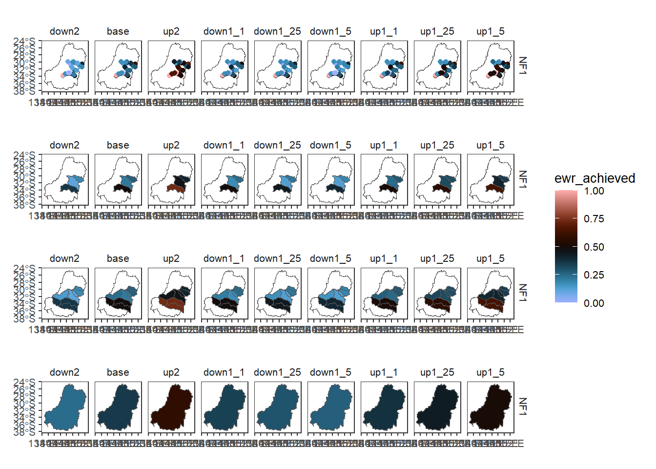
failmissing and keepallpolys
As above, we might want to ignore some groupers or aggregation columns, and we might want to keep polygons that don’t have data so the maps look better.
multispatextra <- multi_aggregate(dat = simpleclean,
                                  causal_edges = themeedges,
                                  groupers = c('scenario', 'env_obj',
                                               'doesnotexist'),
                                  aggCols = c('ewr_achieved', 'notindata'),
                                  aggsequence = glist,
                                  funsequence = funlist,
                                  saveintermediate = TRUE,
                                  namehistory = FALSE,
                                  failmissing = FALSE,
                                  keepAllPolys = TRUE)
We can see that the missing groupers and aggcols get ignored, while we have retained polygons without data. The default is keepAllPolys = FALSE, so the original multispatb only has relevant catchments while multispatextra has all of them. I’ve taken off the basin underlay from the plots above to make this clearer.
keepfalse <- multispatb$catchment %>%
  filter(grepl('^NF1', env_obj) &
           aggfun_1 == 'ArithmeticMean') %>%
  plot_outcomes(y_col = 'ewr_achieved',
                x_col = 'map',
                colorgroups = NULL,
                colorset = 'ewr_achieved',
                pal_list = list('scico::berlin'),
                facet_col = 'scenario',
                facet_row = 'env_obj',
                scene_pal = scene_pal,
                sceneorder = c('down2', 'base', 'up2'),
                setLimits = c(0,1))

keeptrue <- multispatextra$catchment %>%
  filter(grepl('^NF1', env_obj) &
           aggfun_1 == 'ArithmeticMean') %>%
  plot_outcomes(y_col = 'ewr_achieved',
                x_col = 'map',
                colorgroups = NULL,
                colorset = 'ewr_achieved',
                pal_list = list('scico::berlin'),
                facet_col = 'scenario',
                facet_row = 'env_obj',
                scene_pal = scene_pal,
                sceneorder = c('down2', 'base', 'up2'),
                setLimits = c(0,1))
keepfalse / keeptrue + plot_layout(guides = 'collect')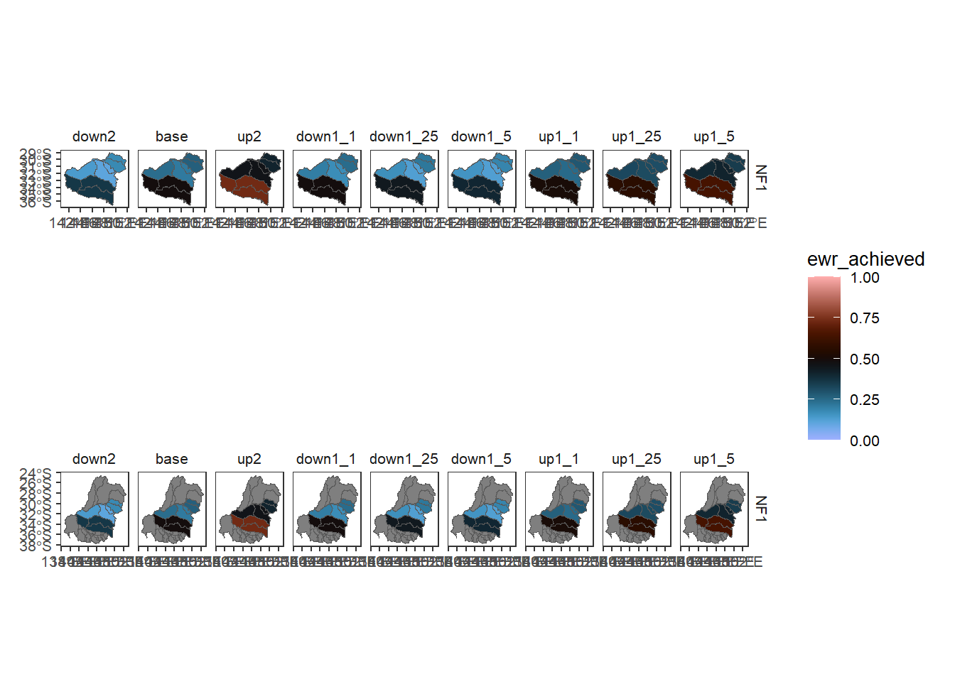
It would be possible to make the same plot by using the catchment polys themselves as underlay, and while the default (underlay_list = 'cewo_valleys' ) would yield white, we also have more control over colour too (not limited to the NA grey).
keepfalse_underlay <- multispatb$catchment %>%
  filter(grepl('^NF1', env_obj) &
           aggfun_1 == 'ArithmeticMean') %>%
  plot_outcomes(y_col = 'ewr_achieved',
                x_col = 'map',
                colorgroups = NULL,
                colorset = 'ewr_achieved',
                pal_list = list('scico::berlin'),
                facet_col = 'scenario',
                facet_row = 'env_obj',
                scene_pal = scene_pal,
                sceneorder = c('down2', 'base', 'up2'),
                underlay_list = list(underlay = 'cewo_valleys',
                                     underlay_pal = 'cornsilk'),
                setLimits = c(0,1))
keepfalse_underlay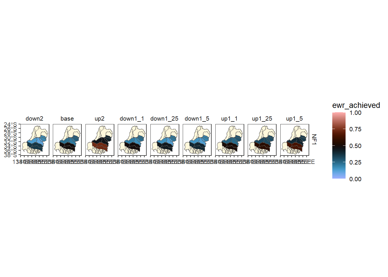
Using multi_aggregate for one aggregation
If we’re only using one level of spatial aggregation and nothing else, there’s typically no need for the multi_aggregate wrapper. That wrapper does work even for single steps though, and becomes almost essential for multi-step. We do have a bit less flexibility with how we specify arguments- aggsequence and funsequence need to be lists or characters (funsequence cannot be bare function names). Perhaps the biggest issue is that tidyselect in aggCols runs into issues because it gets used again inside multi_aggregate, and so tidyselect in the outer call collides with that. That could all be sorted out, but seems low priority- easier to just enforce characters for aggCols and lists or characters for the sequences.
Typically we could use namehistory = FALSE to avoid the horrible long name with all the transforms in it, but there’s no way for it to know the previous aggregation history when it’s been done in pieces (as we say in the example above where I dangerously adjusted the name of simpleThemeAgg to make multispatb. A parsing function could handle this, but it’s better to just do it all on one go anyway so this is low priority.
As a quick example, here is a single-step spatial aggregation using multi_aggregate, not that we have slightly more restrictive specifications for groupers, aggCols, aggsequence and funsequence.
obj2polyM1 <- multi_aggregate(simpleThemeAgg,
                            causal_edges = themeedges,
                            groupers = c('scenario', 'env_obj'),
                         aggCols = 'ewr_achieved',
                         aggsequence = list(sdl_units = sdl_units),
                         funsequence = list(list(am = ~ArithmeticMean(.))),
                         keepAllPolys = TRUE)

obj2polyM1
Next steps
The examples here are designed to dig into capability of the spatial aggregator in fairly high detail. In typical use, we’d follow something more like the interleaved notebook, but this document hopefully provides valuable demonstrations of capability and potential for how each spatial step in that sequence might work and could be set up.